1.1 Introduction
Cost is important to all industry. Costs can be divided into two general classes; absolute costs and relative costs. Absolute cost measures the loss in value of assets. Relative cost involves a comparison between the chosen course of action and the course of action that was rejected. This cost of the alternative action - the action not taken - is often called the "opportunity cost".
The accountant is primarily concerned with the absolute cost. However, the forest engineer, the planner, the manager needs to be concerned with the alternative cost - the cost of the lost opportunity. Management has to be able to make comparisons between the policy that should be chosen and the policy that should be rejected. Such comparisons require the ability to predict costs, rather than merely record costs.
Cost data are, of course, essential to the technique of cost prediction. However, the form in which much cost data are recorded limits accurate cost prediction to the field of comparable situations only. This limitation of accurate cost prediction may not be serious in industries where the production environment changes little from month to month or year to year. In harvesting, however, identical production situations are the exception rather than the rule. Unless the cost data are broken down and recorded as unit costs, and correlated with the factors that control their values, they are of little use in deciding between alternative procedures. Here, the approach to the problem of useful cost data is that of identification, isolation, and control of the factors affecting cost.
1.2 Basic Classification of Costs
Costs are divided into two types: variable costs, and fixed costs. Variable costs vary per unit of production. For example, they may be the cost per cubic meter of wood yarded, per cubic meter of dirt excavated, etc. Fixed costs, on the other hand, are incurred only once and as additional units of production are produced, the unit costs fall. Examples of fixed costs would be equipment move-in costs and road access costs.
1.3 Total Cost and Unit-Cost Formulas
As harvesting operations become more complicated and involve both fixed and variable costs, there usually is more than one way to accomplish a given task. It may be possible to change the quantity of one or both types of cost, and thus to arrive at a minimum total cost. Mathematically, the relationship existing between volume of production and costs can be expressed by the following equations:
Total cost = fixed cost + variable cost × output
![]()
In symbols using the first letters of the cost elements and N for the output or number of units of production, these simple formulas are
C = F + NV
UC = F/N + V
1.4 Breakeven Analysis
A breakeven analysis determines the point at which one method becomes superior to another method of accomplishing some task or objective. Breakeven analysis is a common and important part of cost control.
One illustration of a breakeven analysis would be to compare two methods of road construction for a road that involves a limited amount of cut-and-fill earthwork. It would be possible to do the earthwork by hand or by bulldozer. If the manual method were adopted, the fixed costs would be low or non-existent. Payment would be done on a daily basis and would call for direct supervision by a foreman. The cost would be calculated by estimating the time required and multiplying this time by the average wages of the men employed. The men could also be paid on a piece-work basis. Alternatively, this work could be done by a bulldozer which would have to be moved in from another site. Let us assume that the cost of the hand labor would be $0.60 per cubic meter and the bulldozer would cost $0.40 per cubic meter and would require $100 to move in from another site. The move-in cost for the bulldozer is a fixed cost, and is independent of the quantity of the earthwork handled. If the bulldozer is used, no economy will result unless the amount of earthwork is sufficient to carry the fixed cost plus the direct cost of the bulldozer operation.
Figure 1.1 Breakeven Example for Excavation.
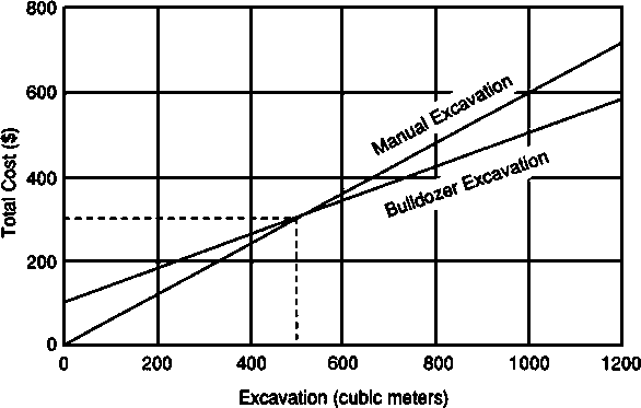
If, on a set of coordinates, cost in dollars is plotted on the vertical axis and units of production on the horizontal axis, we can indicate fixed cost for any process by a horizontal line parallel to the x-axis. If variable cost per unit output is constant, then the total cost for any number of units of production will be the sum of the fixed cost and the variable cost multiplied by the number of units of production, or F + NV. If the cost data for two processes or methods, one of which has a higher variable cost, but lower fixed cost than the other are plotted on the same graph, the total cost lines will intersect at some point. At this point the levels of production and total cost are the same. This point is known as the "breakeven" point, since at this level one method is as economical as the other. Referring to Figure 1.1 the breakeven point at which quantity the bulldozer alternative and the manual labor alternative become equal is at 500 cubic meters. We could have found this same result algebraically by writing F + NV = F' + NV' where F and V are the fixed and variable costs for the manual method, and F' and V' are the corresponding values for the bulldozer method. Since all values are known except N, we can solve for N using the formula N = (F' - F) / (V - V')
![]()
1.5 Minimum Cost Analyses
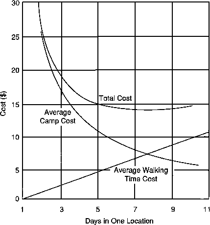
A similar, but different problem is the determination of the point of minimum total cost. Instead of balancing two methods with different fixed and variable costs, the aim is to bring the sum of two costs to a minimum. We will assume a clearing crew of 20 men is clearing road right-of-way and the following facts are available:
1. Men are paid at the rate of $0.40 per hour.
2. Time is measured from the time of leaving camp to the time of return.
3. Total walking time per man is increasing at the rate of 15 minutes per day.
4. The cost to move the camp is $50.
If the camp is moved each day, no time is lost walking, but the camp cost is $50 per day. If the camp is not moved, on the second day 15 crew-minutes are lost or $2.00. On the third day, the total walking time has increased 30 minutes, the fourth day, 45 minutes, and so on. How often should the camp be moved assuming all other things are equal? We could derive an algebraic expression using the sum of an arithmetic series if we wanted to solve this problem a number of times, but for demonstration purposes we can simply calculate the average total camp cost. The average total camp cost is the sum of the average daily cost of walking time plus the average daily cost of moving camp. If we moved camp each day, then average daily cost of walking time would be zero and the cost of moving camp would be $50.00. If we moved the camp every other day, the cost of walking time is $2.00 lost the second day, or an average of $1.00 per day. The average daily cost of moving camp is $50 divided by 2 or $25.00. The average total camp cost is then $26.00. If we continued this process for various numbers of days the camp remains in location, we would obtain the results in Table 1.1.
TABLE 1.1 Average daily total camp cost as the sum of the cost of walking time plus the cost of moving camp.
|
Days camp remained in location |
Average daily cost of walking time |
Average daily cost of moving camp |
Average total camp cost |
|
1 |
0.00 |
50.00 |
50.00 |
|
2 |
1.00 |
25.00 |
26.00 |
|
3 |
2.00 |
16.67 |
18.67 |
|
4 |
3.00 |
12.50 |
15.50 |
|
5 |
4.00 |
10.00 |
14.00 |
|
6 |
5.00 |
8.33 |
13.33 |
|
7 |
6.00 |
7.14 |
13.14 |
|
8 |
7.00 |
6.25 |
13.25 |
|
9 |
8.00 |
5.56 |
13.56 |
|
10 |
9.00 |
5.00 |
14.00 |
We see the average daily cost of walking time increasing linearly and the average cost of moving camp decreasing as the number of days the camp remains in one location increases. The minimum cost is obtained for leaving the camp in location 7 days (Figure 1.2). This minimum cost point should only be used as a guideline as all other things are rarely equal. An important output of the analysis is the sensitivity of the total cost to deviations from the minimum cost point. In this example, the total cost changes slowly between 5 and 10 days. Often, other considerations which may be difficult to quantify will affect the decision. In Section 2, we discuss balancing road costs against skidding costs. Sometimes roads are spaced more closely together than that indicated by the point of minimum total cost if excess road construction capacity is available. In this case the goal may be to reduce the risk of disrupting skidding production because of poor weather or equipment availability. Alternatively, we may choose to space roads farther apart to reduce environmental impacts. Due to the usually flat nature of the total cost curve, the increase in total cost is often small over a wide range of road spacings.
Figure 1.2 Costs for Camp Location Example.